Open source · MATLAB
github.com/muhammadzareii/coupled-qw-valence-bandOverview
In a bulk semiconductor, the valence band near the Γ-point splits into three sub-bands: heavy hole (HH), light hole (LH), and spin-orbit split-off. When the semiconductor is grown as a quantum well (QW), the quantum confinement breaks the degeneracy between HH and LH at k = 0, and the in-plane wave-vector couples them through the Luttinger-Kohn (L-K) Hamiltonian. This mixing — known as band mixing or k·p coupling — has significant implications for optical gain, polarisation selection rules, and intersubband absorption in optoelectronic devices.
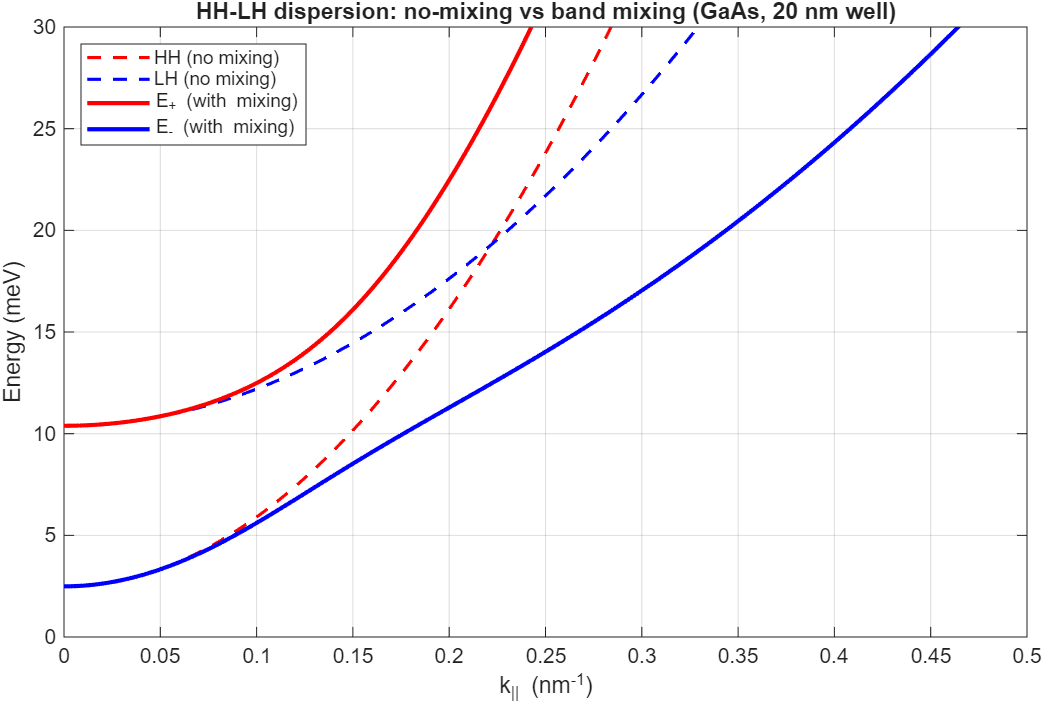
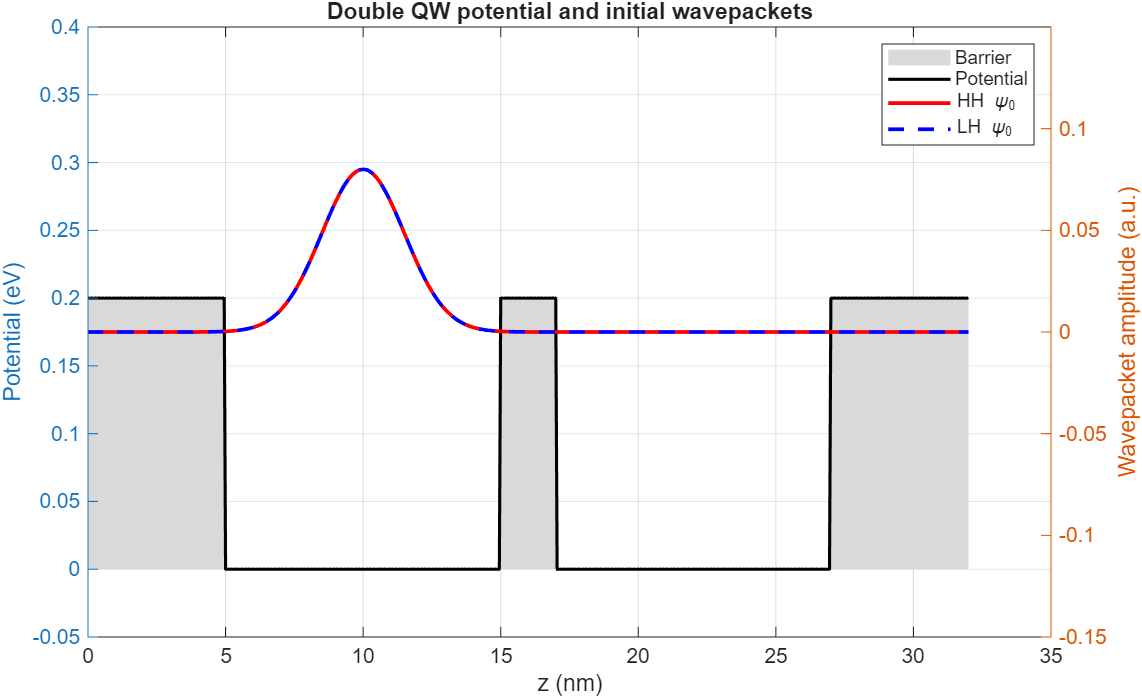
This project solves the L-K Hamiltonian for a GaAs/Al₀.₅Ga₀.₅As double quantum well (two coupled 25 Å wells separated by a 15 Å barrier), computes the HH and LH energy subband dispersion as functions of in-plane wavevector k∥, and simulates the time evolution of Gaussian wavepackets initialised in each subband. The coupling between HH and LH states is visible in the oscillatory probability density transfer between wells as the wavepacket evolves.
Structure Parameters
| Parameter | Value |
|---|---|
| Well material | GaAs |
| Barrier material | Al₀.₅Ga₀.₅As |
| Well width (each) | 25 Å (2.5 nm) |
| Barrier width | 15 Å (1.5 nm) |
| Valence band offset ΔE_v | 0.25 eV |
| Luttinger parameters γ₁, γ₂ | GaAs: γ₁ = 6.98, γ₂ = 2.06; AlGaAs: interpolated |
| Wavepacket initial condition | Gaussian envelope in z, zero in-plane momentum |
Luttinger-Kohn Hamiltonian
The 4×4 Luttinger-Kohn Hamiltonian (for spin up/down HH and LH) in the growth direction (z) is:
(γ₁ + γ₂)k_z² −√3·γ₂·k_−² −√3·γ₃·k_z·k_− 0
−√3·γ₂·k_+² (γ₁ − γ₂)k_z² 0 −√3·γ₃·k_z·k_+
−√3·γ₃·k_z·k_+ 0 (γ₁ − γ₂)k_z² √3·γ₂·k_−²
0 −√3·γ₃·k_z·k_− √3·γ₂·k_+² (γ₁ + γ₂)k_z² ]
where k_± = k_x ± ik_y are the in-plane wavevectors. In the 1D problem (k∥ = 0 at the subband minimum) the off-diagonal terms vanish and HH/LH decouple, giving analytically solvable confinement energies. At finite k∥, the coupling mixes the states, creating the characteristic anti-crossing dispersion.
Results