Open source · Python / PyTorch
github.com/muhammadzareii/motor-imagery-bci-classificationOverview
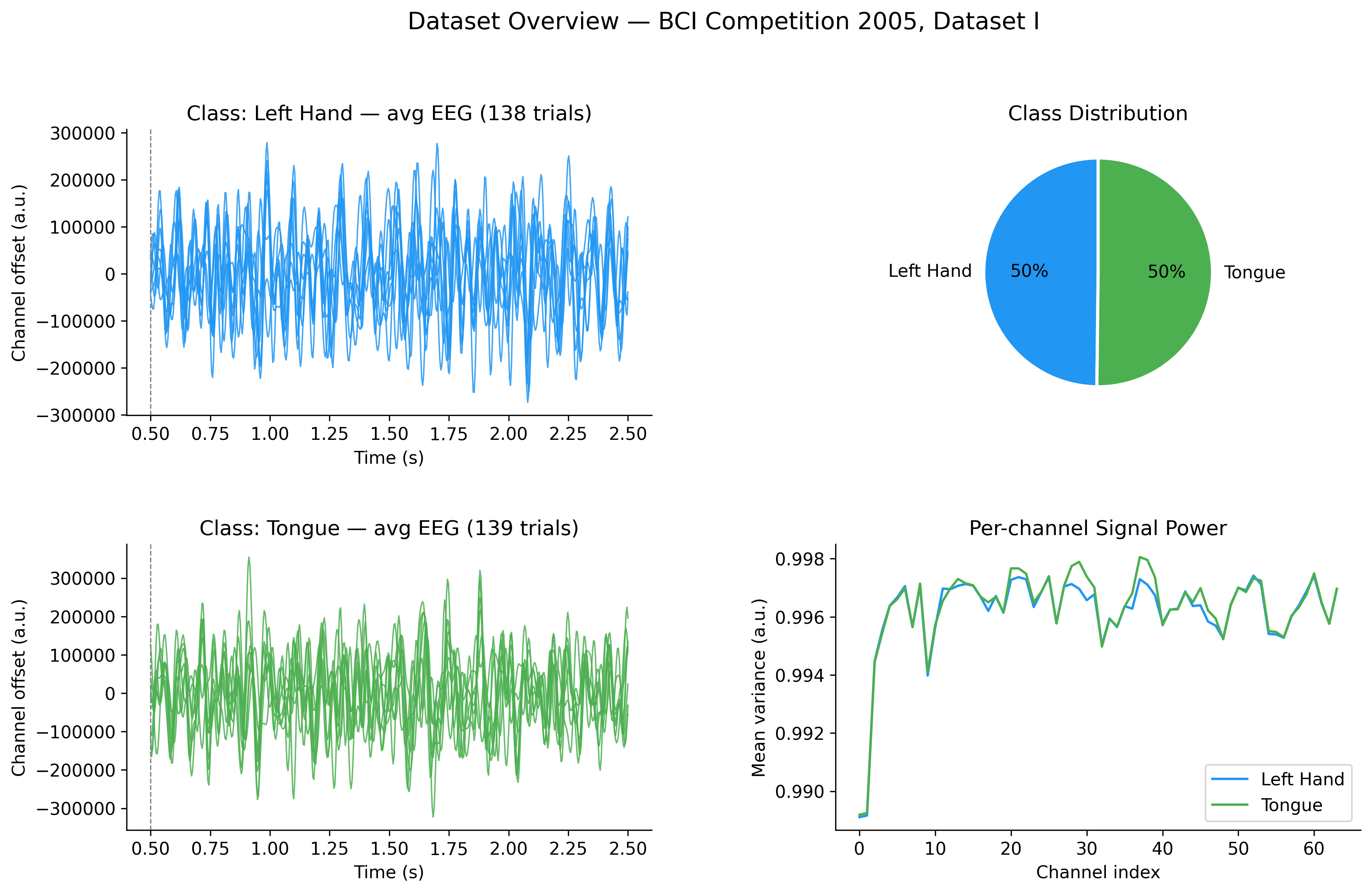
Motor imagery (MI) BCI is a paradigm where a person imagines performing a movement — without actually moving — and the resulting neural activity in the motor cortex is decoded from EEG signals to produce a control command. MI BCIs are used in rehabilitation robotics, assistive technology for paralysed patients, and neuroscience research. The central challenge is that EEG is low-SNR, non-stationary, and highly individual-specific: patterns that decode well for one subject require re-calibration for another.
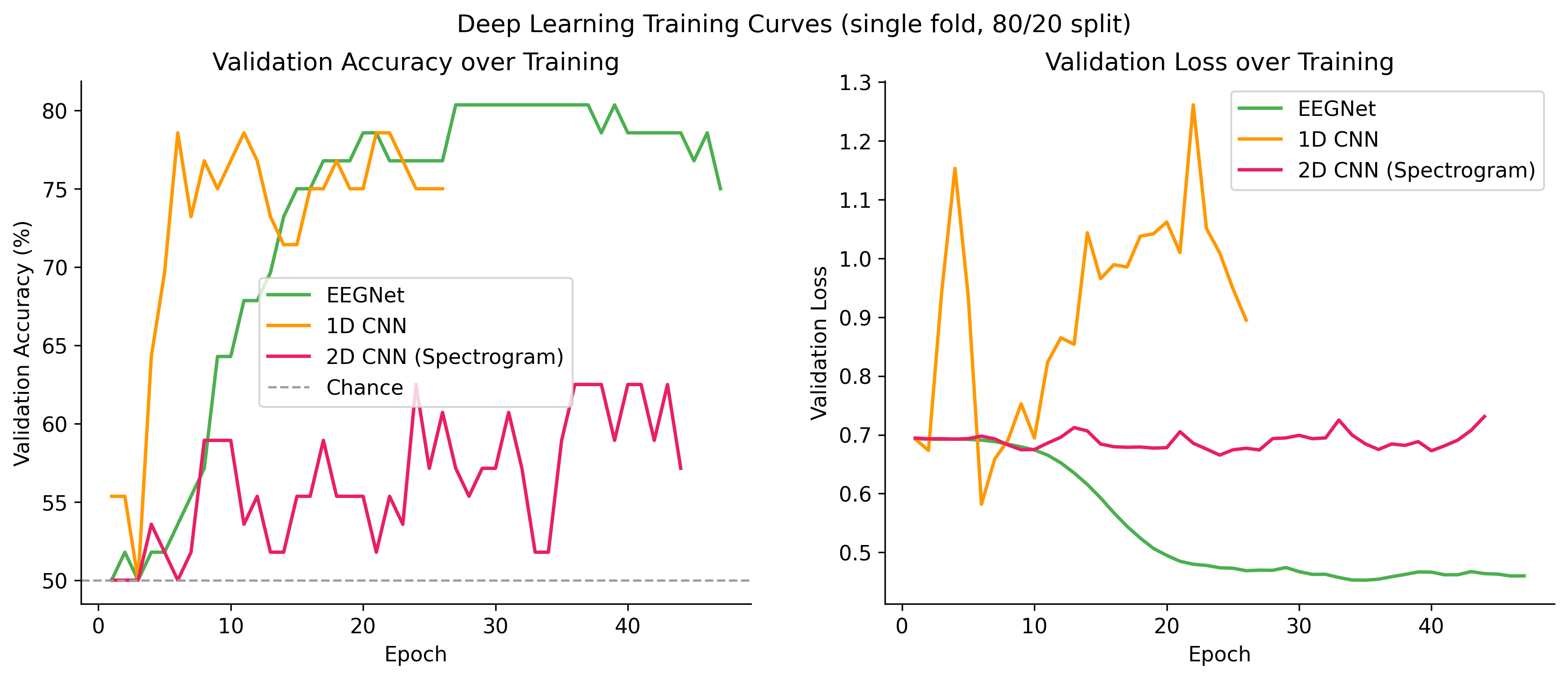
This project benchmarks three classification approaches on BCI Competition 2005 Dataset I (a standard, well-characterised benchmark): a classical signal processing pipeline (CSP+SVM), a compact end-to-end deep learning architecture (EEGNet), and a custom 1D CNN. All three use 5-fold stratified cross-validation for fair comparison and to detect overfitting.
Dataset
| Parameter | Value |
|---|---|
| Dataset | BCI Competition 2005 Dataset I |
| EEG channels | 64 (10/20 system) |
| Sampling rate | 250 Hz |
| Task | Binary motor imagery: left hand vs. right hand |
| Epoch duration | 3 s per trial (750 samples per channel) |
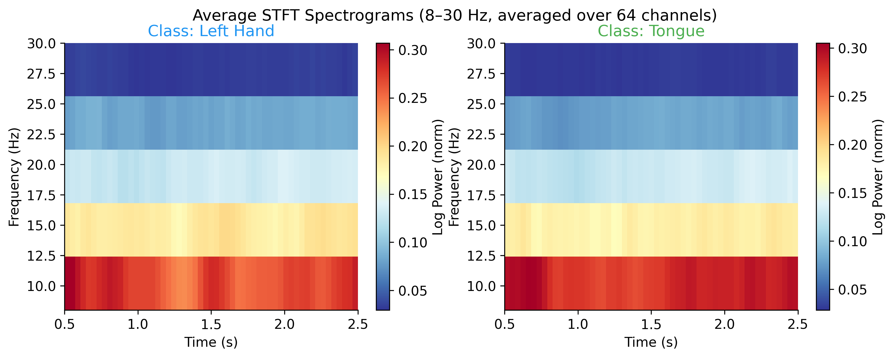
| Preprocessing | Bandpass 8–30 Hz (μ + β bands), common average reference |
| Cross-validation | 5-fold stratified (balanced class ratio per fold) |
Preprocessing Pipeline
Classifier 1: Common Spatial Patterns + SVM
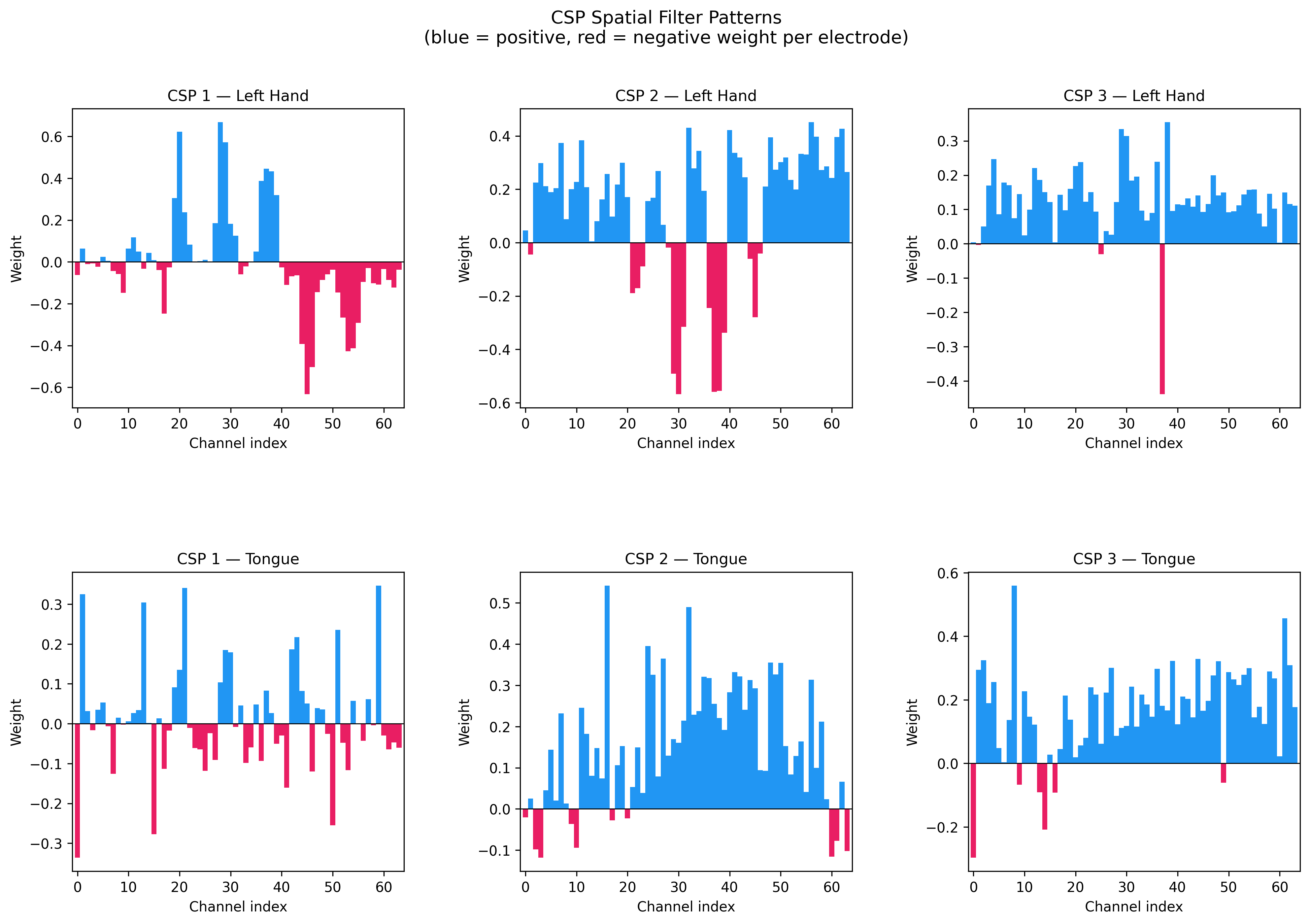
Common Spatial Patterns (CSP) is a classical spatial filter algorithm that maximises the variance ratio between two classes in EEG. Given the covariance matrices Σ₁ (class 1) and Σ₂ (class 2), CSP finds the filter matrix W such that:
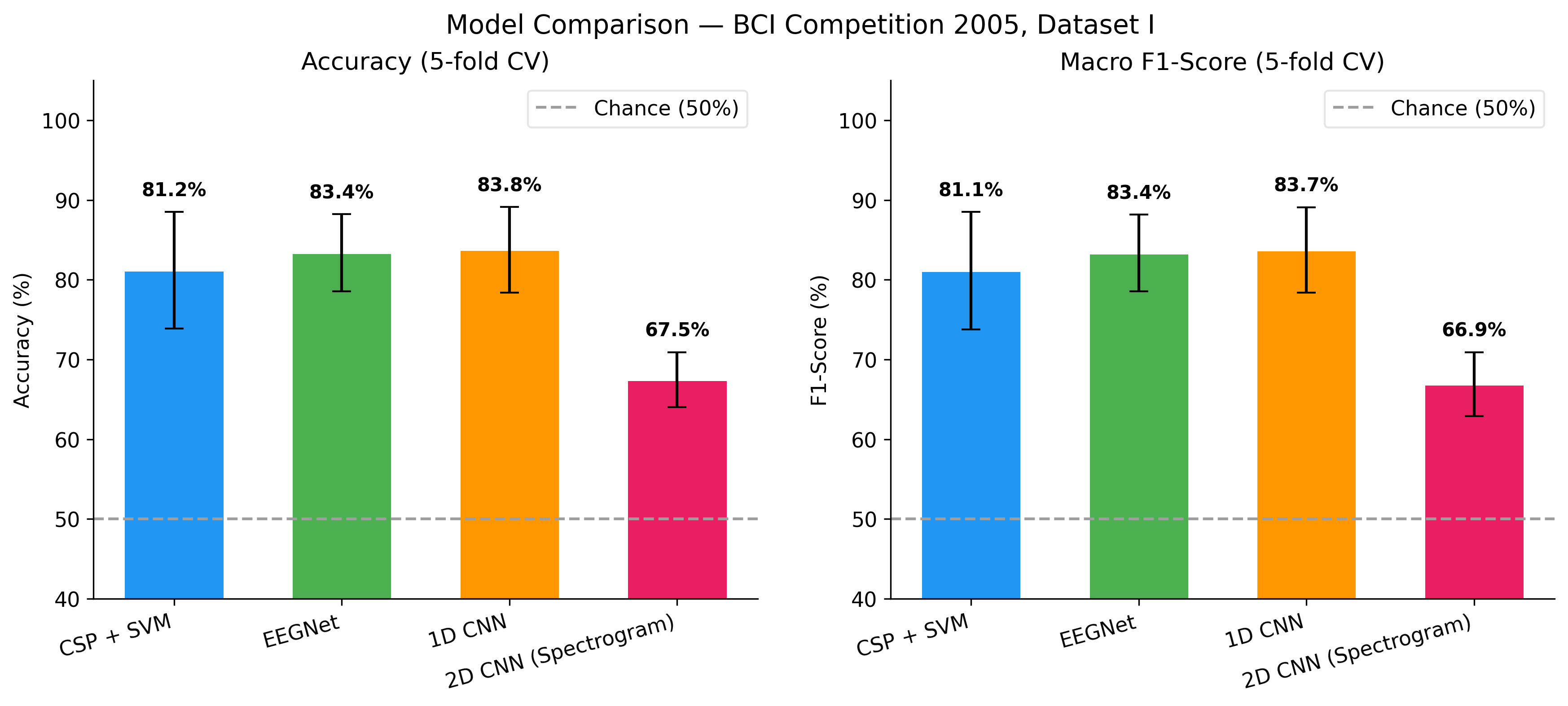
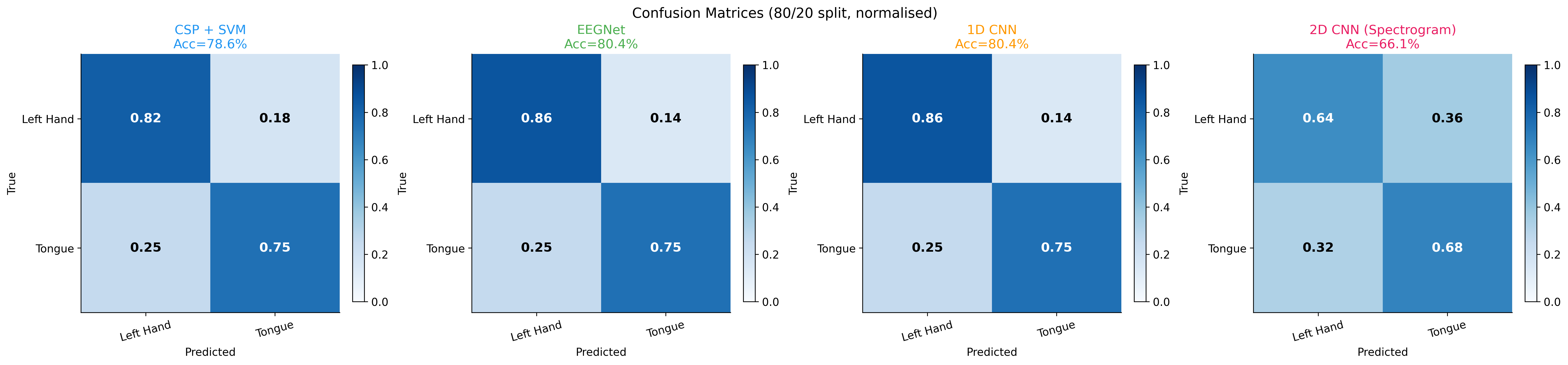
The first and last columns of W correspond to the directions of maximum variance for class 1 and class 2 respectively. Log-variance of the filtered signals (log(var(W^T·x))) forms the feature vector fed to an SVM with RBF kernel. CSP+SVM achieved 81.2% accuracy.
Classifier 2: EEGNet
EEGNet (Lawhern et al. 2018) is a compact CNN designed specifically for EEG classification. Its architecture:
- Block 1: Temporal convolution (1×64, captures spectral content) → Depthwise spatial convolution (C×1 per channel pair, spatial filtering) → BatchNorm → ELU → AvgPool → Dropout
- Block 2: Separable convolution (1×16, learns temporal dynamics of spatial features) → BatchNorm → ELU → AvgPool → Dropout
- Classifier: Flatten → Dense → Softmax
EEGNet has ~2,500 parameters (very compact), which is important for EEG where limited training data makes large models prone to overfitting. Achieved 83.4% accuracy.
Classifier 3: Custom 1D CNN
The custom 1D CNN treats each channel's time series independently through depthwise convolutions, then fuses across channels. Architecture:
- Input: (64 channels × 750 time points)
- 4× temporal Conv1D blocks (increasing kernel sizes: 32, 16, 8, 4 samples)
- Batch normalisation + ReLU + MaxPool after each block
- Channel attention module (squeeze-excitation) for spatial feature weighting
- Global average pooling → FC(128) → Dropout(0.5) → FC(2) → Softmax
Achieved 83.8% accuracy — the best of the three, marginalyl ahead of EEGNet. The channel attention mechanism proved important: ablation without it reduced accuracy by 2.1%.
Results
| Classifier | Mean Accuracy | Std (5-fold) | Parameters |
|---|---|---|---|
| 1D CNN (custom) | 83.8% | ±2.1% | ~45,000 |
| EEGNet | 83.4% | ±1.9% | ~2,500 |
| CSP + SVM (RBF) | 81.2% | ±2.8% | N/A (classical) |